by Fabio Andrijauskas, Igor Sfiligoi and Frank Wüerthwein - University of California San Diego, as of January 7, 2022

Open Science Grid (OSG) has a complex system to access all the available resources. Figure 1 shows a vision of HTCondor and glidein Workflow Managment System (GlideinWMS) how they provide access to the computer structure [1].

Figure 1 shows the main idea is that when demand for more resources is sensed by the Virtual Organization Frontend, Condor job execution daemons (aka glidein pilots) are submitted to the grid by the Glidein Factory (GF):

Even with this well-made structure, it is a fact of life that the resources are not always perfectly utilized. In order to improve utilization of the available resource, we first must have a clear understanding of how to classify the activity of those resources.

For this proposal, we are concerned only about wall time measures due to the combined gWMS and HTCondor systems. The proposed classification thus may be understood largely as a walk through the "state machine" of how these two systems work together.

Note that we will be considering CPU and GPU resources separately for ease of understanding. We thus define the unit of “time” as “cpu core hours” for CPUs and “gpu chip hours” for GPUs.

Moreover, to account for the fine-grained partitioning inside pilot jobs, we also define a notion of “canonical unit”. At this point in time, we propose to define it as “1 CPU core + 2 GB of RAM” for CPU resources and “1 GPU chip” for GPU resources. It can then be used to compute “canonical time” in the same units as normal time. The detailed use of this unit is discussed below.

We postulate that the time of resources available to OSG can be partitioned among the following 8 categories, with the first 6 belonging to the pilot infrastructure:

• Validation fail: Any time spent by a pilot that failed the initial validation (so the collector was never aware of it).

• Decision problem: Any time spent by a pilot that starts and registers with the collector but does not get any match before the pilot end of life (EOF).

• Pilot misconfiguration badput: Any time spent by a pilot running jobs that fail in the beginning due to a runtime problem not imputable to user errors (e.g. black hole).

  While the definition is necessarily somewhat ambiguous, the intention is to capture any resource hardware or configuration problems that should have been caught by validation.

• Pilot goodput: Any time spent by a pilot running jobs that complete.

  Note that we do not check the exit code of the job and do not attempt in any way to interpret the outcome from the user point of view. Any job that starts and finishes on its own is considered successful, with the limited exception of the “pilot misconfiguration badput” definition.

• Pilot preemption badput: Any time spent by jobs that start running but do not finish because the pilot terminates (end of life).

• Pilot overhead: For any pilot that starts at least one job, any canonical time spent not running any jobs is counted as pilot overhead. Any difference between “total time” and “canonical time” will instead be proportionally accounted to any jobs running at that time, if any.

  Further clarification and some examples regarding the accounting using canonical time is presented below in a dedicated paragraph.

  Note that any time spent before the first job is ran is accounted to either (1) or (2), if the pilot never runs a single job, and here else.

• Pilot goodput: Any time spent by a pilot running jobs that complete.

  Note that we do not check the exit code of the job and do not attempt in any way to interpret the outcome from the user point of view. Any job that starts and finishes on its own is considered successful, with the limited exception of the “pilot misconfiguration badput” definition.

• Pilot preemption badput: Any time spent by jobs that start running but do not finish because the pilot terminates (end of life).

There are two additional classifications of time available to OSG and not directly related to pilot infrastructure:

• Provisioning bottleneck: Any time a resource provider, aka site, is sitting idle because we did not send enough pilots, even though we had user jobs waiting for resources.

• Insufficient demand: Any time a resource provider, aka site, is sitting idle because we did not send enough pilots because there are no jobs waiting that can run on that resource.

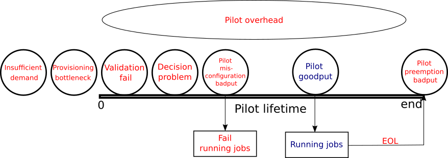
Figure 2 shows a simplified pilot's lifetime and when each type of measure happens.

Further clarification of “Pilot overhead” and canonical units

OSG jobs come with fine-grained requirements, while the pilots offer a fixed total number of CPU cores, GPUs, and memory, and there is no optimal way to maximize the use of all the resources while keeping job priorities in consideration. OSG thus allows for certain resources to be idle, if some of the other equally important resources are fully utilized. For example, it is just as acceptable to “use all the CPU cores and only a fraction the memory” as it is to “use all the memory and only a subset of the CPU cores”.

The “canonical unit” and “canonical time” definitions provide a measure of what is the smallest unit that is considered “true overhead”. We thus account “Pilot overhead” only in multiples of “canonical units”. For example, given the CPU definition of canonical unit of “1 CPU core and 2 GB of memory”, an hour when we have 3 CPU cores and 3 GB of memory unused would count as “1 CPU core hour” (memory limited), the same period of 3 CPU cores and 1 GB of memory unused would count as “0 CPU core hours” (memory limited), and the same period of 2 CPU cores and 6 GB of memory unused would count as “2 CPU core hours” (CPU core limited).

The use of “canonical time” in “Pilot overhead” brings however an accounting problem; I.e. What to do with the remainder of the time that remains unaccounted for. Using the first example above, when we have 3 CPU cores and 3 GB of memory unused, we have a remainder of “2 CPU core hours”.

In order to fully account for all the resources, we thus account that remainder proportionally between any jobs that were running at that point in time. For example, if we had a remainder of 2 CPU cores (and any amount of memory) and there were two jobs running during the considered time period, say 1h for example simplicity, one which completed and one that never did due to the pilot getting preempted sometime in the future, we would account 1 CPU core hour to each of “Pilot goodput” and “Pilot preemption badput”. As a further clarification, any time the pilot does not run any jobs at all, all the time is accounted to “Pilot overhead”, even if it is not a multiple of “canonical time”.

Note that for GPU accounting “canonical time” is currently defined the same as “time”, i.e. “GPU chip hours”, so there is never any leftover there.

A word about time classification vs measurement:

This document only provides the partitioned definitions of how the resources are being used. It does not aim to provide any guidance regarding how to classify the resource usage using the existing monitoring tools.

As an example, it is currently unknown how to properly measure (a) and (b) but one could speculate that one could approximate it by means of measuring period with no pilots waiting in the sites’ queues. Such clarifications and guidance are of course necessary but will be subject to a separate future document.