Throughput Machine Learning with Heterogeneous resources - Final Report
PATh Supplement - Status and Progress of Heterogeneous Model Training
Executive Summary
This project investigates the feasibility and reviews the experience of training machine learning model ensembles across heterogeneous resources from a single HTCondor access point (AP). These resources are spatially separated and exist across multiple computing ecosystems, using both the OSPool and resources granted through the NAIRR Pilot Program. We trained 33 complete (30 epoch) versions of a METL protein language model across two different model architectures. With additional (ongoing) training runs, this amounts to 1,266 epochs of training total, consuming over 23,273 GPU hours on 10 different GPU models. Our results show that model training is robust in a heterogeneous environment, and that the PATh services, backed by the HTCondor and Pelican software, provide suitable tools for submitting and managing the training process. However, there are workflow challenges that have been identified as well, especially in terms of full automation. Performance variability indicate site-specific factors that can impact training performance. Overall, this work shows that the PATh ecosystem is a technically viable solution for training ensembles of models that are easily checkpointable and fit within small to moderate GPU needs.
Key Findings
-
Heterogeneous training across OSPool and NAIRR-allocated sites is technically feasible from a single HTCondor access point, with OSDF used to move the container image and training data to each site.
-
33 complete METL training runs (1,266 epochs, over 23,273 GPU hours across 10 GPU models) were completed without loss of scientific validity.
-
Heterogeneous and homogeneous (single-site) training convergje to comparable final test loss and Pearson total score, though the heterogeneous approach shows higher variability within each epoch evaluation.
-
The main automation gap is HTCondor Annex re-establishment, which currently requires manual, two-factor-authenticated intervention when a site’s annex expires between uses.
-
A new Annex version and an NDJSON-based provenance tracking system are in progress to support ongoing work and to address logging and reportin gaps.
Objectives
As a supplement to the Partnership to Advance Throughput Computing (PATh) project, we have launched a collaboration with a group of domain scientists and ML researchers to run a pathfinder project profiling the effects of distributed and heterogeneous capacity on throughput training and inference computing processes. The goals of this activity are:
-
Characterize the impact of training ensembles across heterogeneous resources, as opposed to the traditional approach of working within a “single homogeneous cluster”.
-
Use the workloads developed in (1) to improve capabilities and services, reducing the barrier of entry for new ML researchers to use the PATh resources to train ensembles, with additional capacity powered by the NAIRR pilot.
-
Demonstrate running single workloads managed by a single AP effectively across as many of the NAIRR pilot resources as possible.
To accomplish these goals, we used the existing Gitter lab’s published Mutational Effect Transfer Learning (METL) protein language model1, using existing data and software to train a modest number of model variants (20-30) from a single AP, intentionally moving the training processes between available resources at training epoch boundaries. Comparison of these variants will prove compatibility of the models, ensuring that the heterogeneity of resources did not impact the scientific power of the models. A second round of experiments, leveraging a larger “global” model architecture was also conducted to test the feasibility of training larger models, requiring approximately 60 GB of GPU memory.
Methodology
NAIRR allocations
Through the NAIRR pilot program, we applied (NAIRR240335) for and received allocations at 6 sites:
| Site | Approved allocation |
|---|---|
| NCSA Delta GPU | 11,500 GPU hours |
| Amazon Web Services | $6,300 |
| Indiana Jetstream2 GPU | 86,016 SUs |
| PSC Bridges-2 GPU | 1,500 GPU hours |
| Purdue Anvil GPU | 1,500 GPU hours |
| SDSC Expanse GPU | 1,500 GPU hours |
In September of 2025, we requested, and received, an additional 2,000 GPU hours from each of Bridges-2, Anvil, and Expanse to account for the increased need from the second round of experiments. We have filed for multiple time extensions in order to continue to run experiments on allocations.
Access Point
We used the OSPool access point ap40.uw.osg-htc.org for all training jobs targeting either OSPool or NAIRR resources. The second round of experiments included baseline runs run within CHTC, ap2002. There is no special configuration needed on the shared access points to enable utilization of the NAIRR resources beyond the pre-existing configuration to enable HTCondor Annex creation.
Job description
The METL software is well-documented with publicly available sourcecode (https://github.com/gitter-lab/metl/). Input data and conda environments are similarly available within Zenodo2. In order to ease the distribution and deployment of the training software, a Docker container image was created (https://github.com/CHTC/METL-Conductor/blob/main/Dockerfile) which contains the installed software. This image was then converted into an apptainer3 image. The apptainer and input data were then stored in the OSPool staging area via OSDF in order to ease the movement across the computing ecosystem. Total input sizes are ~6GB for the image and ~20GB for the data.
Initial benchmarking of the training task was first tested locally on V100 machines, giving approximate resource needs. Additional benchmarking was done both in the CHTC and OSPool clusters to further test and understand the performance and resource needs of the training process.
Finally, test jobs were run within the targeted NAIRR sites to comb out the differences between the sites and to dial in the resource requirements within the job definitions needed for each.
HTCondor Annex
In order to provide single-AP access to the NAIRR sites, we used HTCondor’s Annex feature. This tool submits a pilot job (or jobs) into a remote site based on the resource requests and desired number of nodes from the researcher. These jobs use the sites’ local scheduling software and, upon starting, will create an HTCondor Execution Point (EP) that become available within the researcher’s local cluster to run their job lists.
Minor development was needed within the annex software, primarily to update the partition definitions and settings at the remote sites. The AWS annex required additional development to run an Amazon Machine Image (AMI) compatible with GPU usage.
DAG
We built upon a previous summer fellow’s work to create a suite of tools to create and monitor Direct Acyclic Graph (DAG) workflows that use HTCondor’s DAGMan feature. The workflow generation process sought to:
-
Organize and automate the trianing workload\
-
Identify common patterns of scripted DAG generation\
-
From 2, understand the shortcomings of DAGMan within the context of throughput training tasks (ensemble training or hyperparameter sweeps, for example)
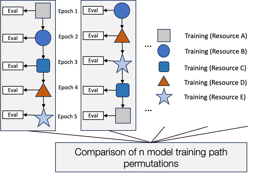
The DAG itself is an array of “shish-kebab” subgraphs, with each stack defining the training process of one model variant. Each of these training runs had run-specific information (an unique identifier, random seed, and the desired number of training epochs). Each node within the graph defines a single job, itself describing a single epoch of training.
Monitoring
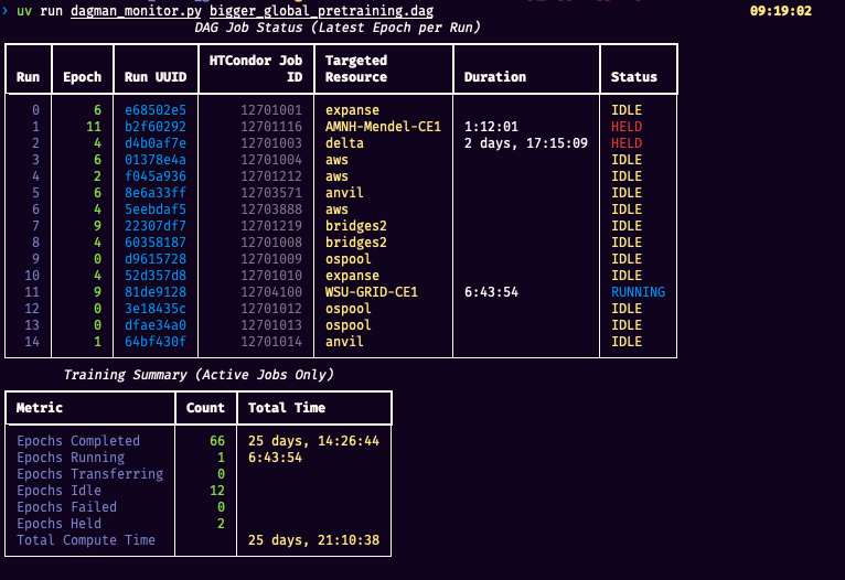
In order to monitor the training processes, a script was developed that tails HTCondor logs, DAGMan logs, and the DAG definition files to provide an overview of how training runs are progressing. By default, it shows the most recent (in-progress or idle) epoch within each training run, displaying the HTCondor job ID, the targeted resource, its current state (idle, transferring, running, held, complete), and the time spent in the current state. It also provides a global summarization of the total number of epochs trained across all runs, along with the number of epochs in each state. Finally, it provides a summary of the total time spent in computation across all training runs. See Figure 2 for a screenshot of the utility.
Additionally, the tool can provide per-training run summaries, showing where each epoch was completed and the amount of execution time taken. There is also a collection of post-processing and analysis scripts to report on overall behavior of the training process.
Experiment 1: Initial METL Model Training
Model configuration
The initial round of experiments was run on a METL-Local model. This is a transformer encoder with 3 layers, 4 attention heads, embedding dimension 256, and feedforward width 1024, resulting in 2.4M total parameters. This model is intended to be trained on a single protein structure and some variants, but during validation, it was discovered that this the dataset used for training was unintentionally the “global” dataset. This dataset, a collection of Rosetta4 simulations containing a wide variety of protein structures and variants, is too large and varied to be used as useful input to this model architecture. However, the training process itself was still informative in our experiments, so is included here.
Results
Training process
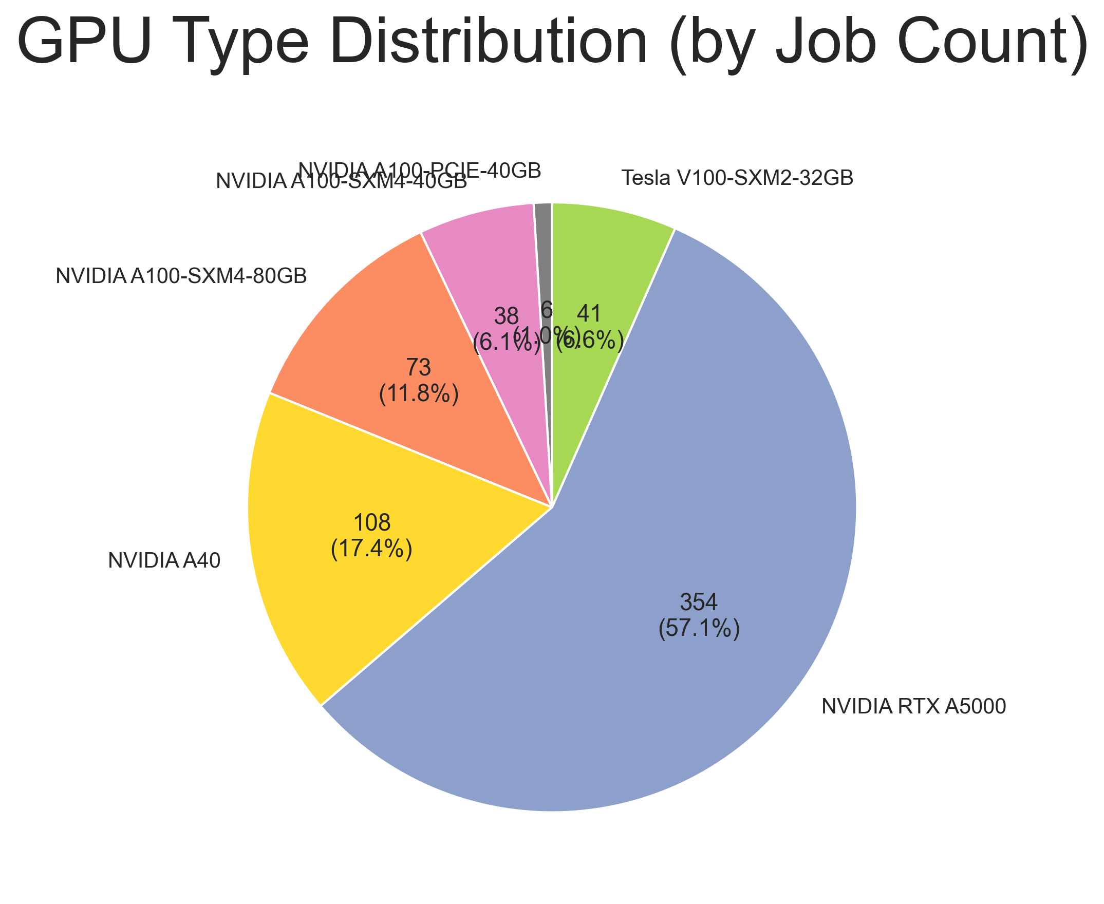
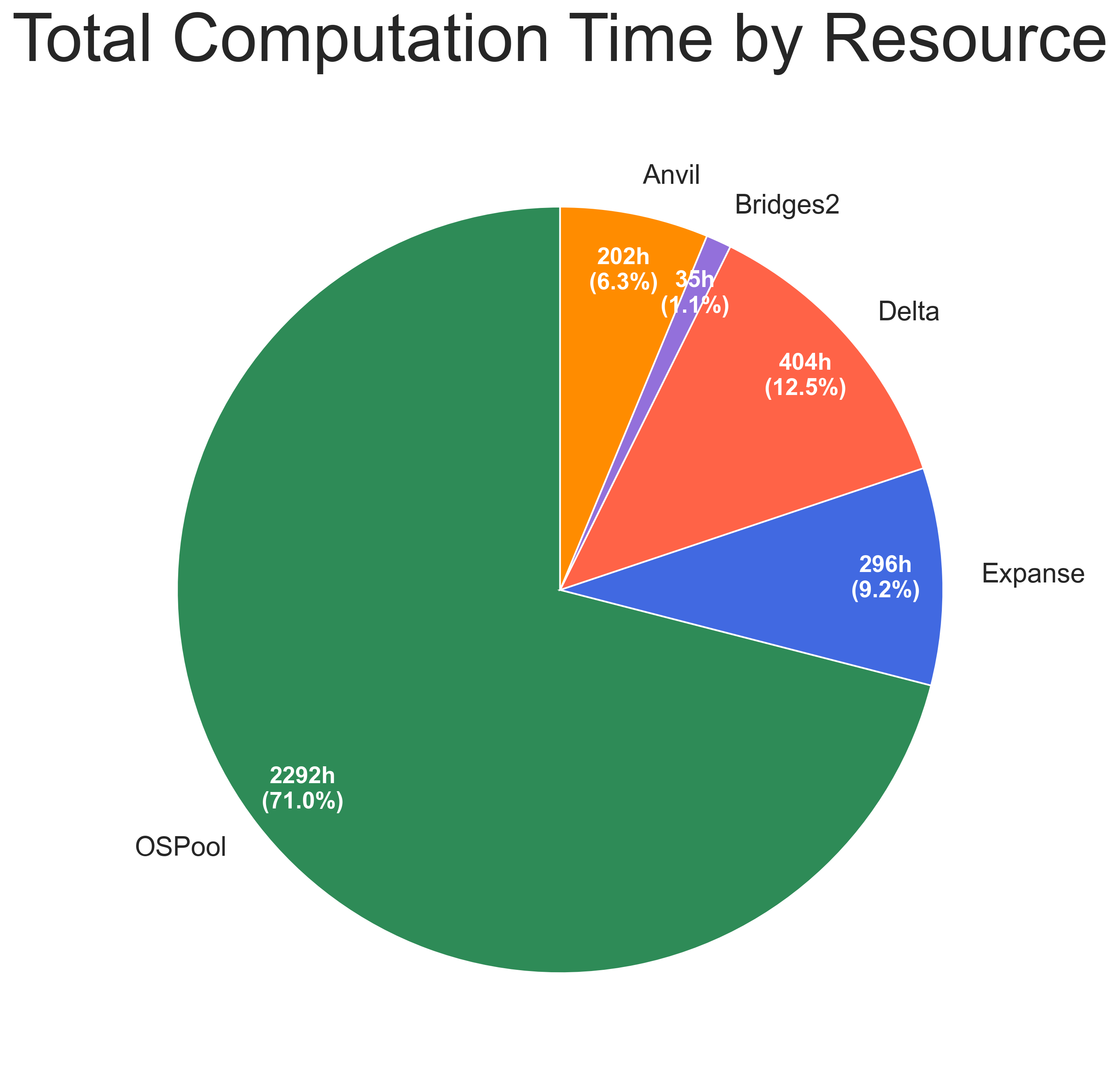
In total, 5,318.6 GPU hours were utilized Six different GPU models were utilized:
| GPU Model | Epochs trained |
|---|---|
| A100-PCIE-40GB | 6 |
| A100-SXM4-40GB | 43 |
| A100-SXM4-80GB | 73 |
| A40 | 108 |
| RTX A5000 | 354 |
| V100-SXM2-32GB | 46 |
GPU Utilization Breakdown
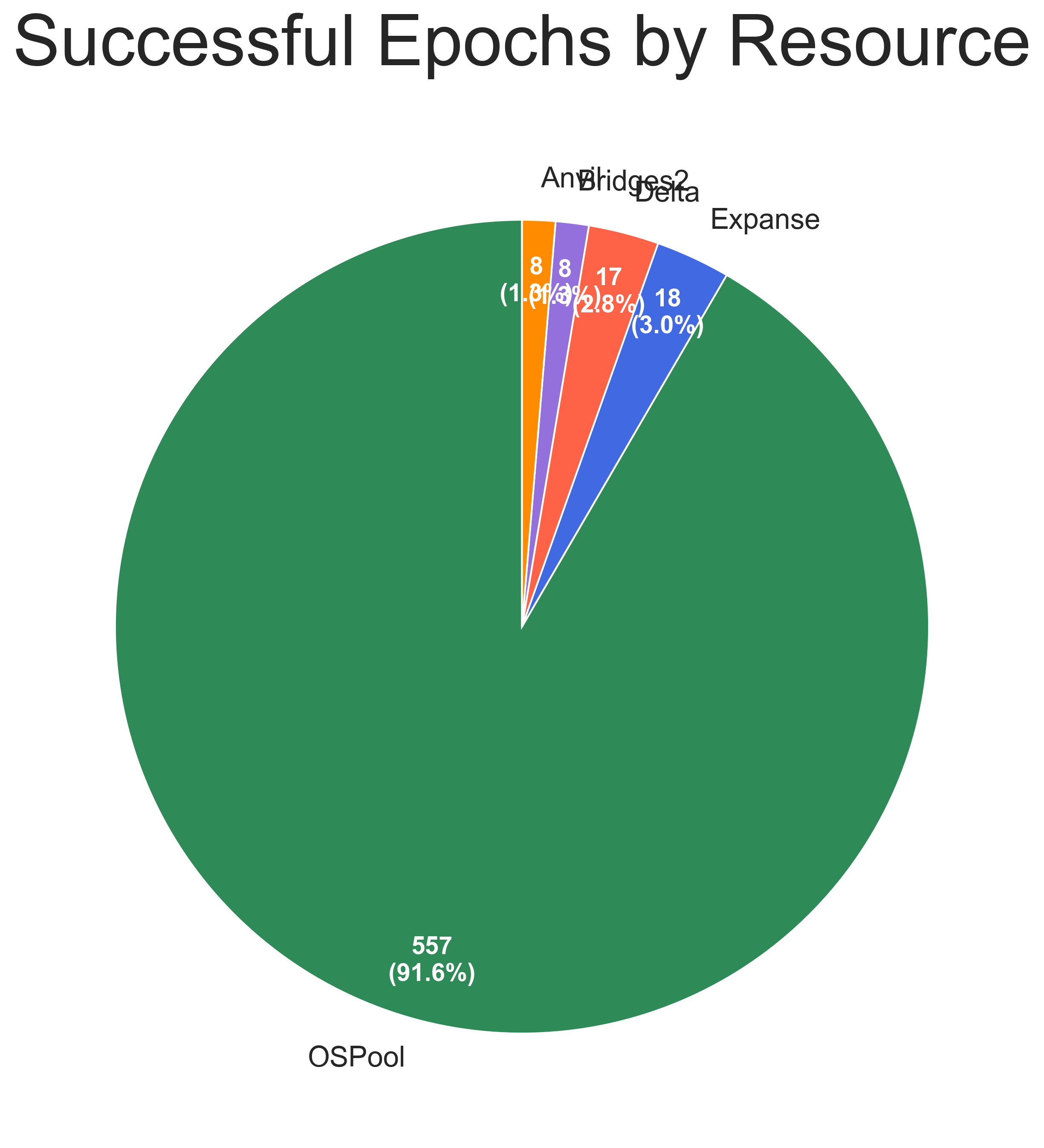
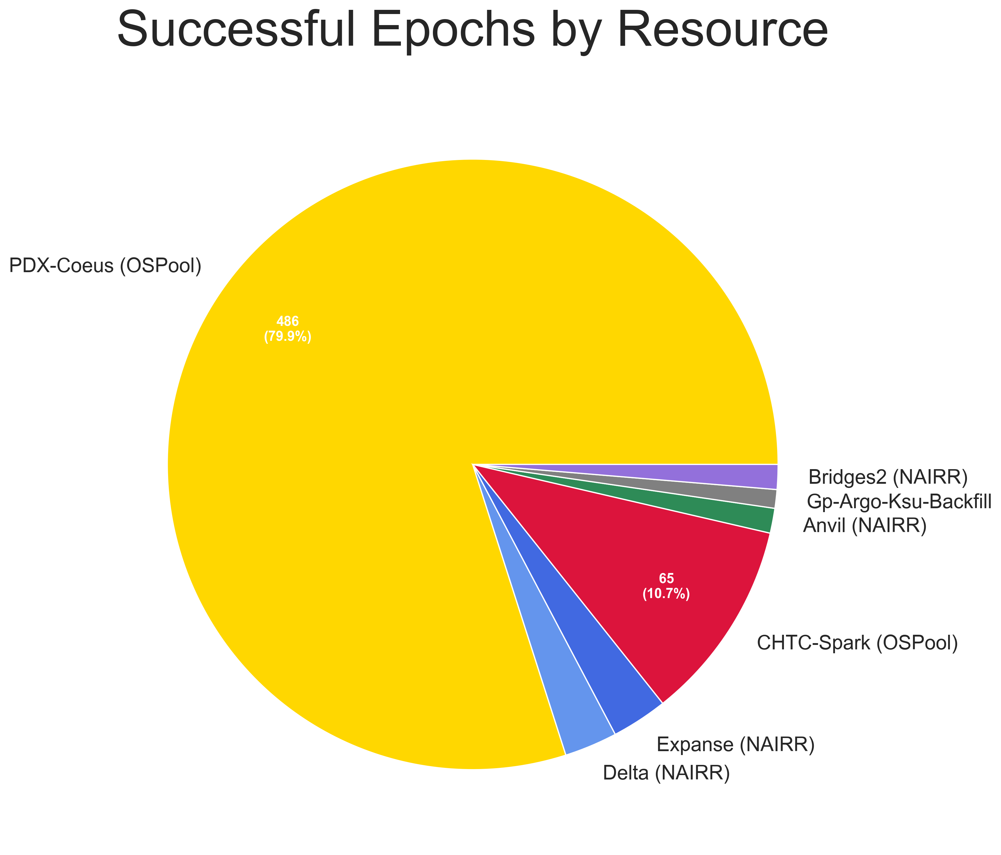
Evaluation
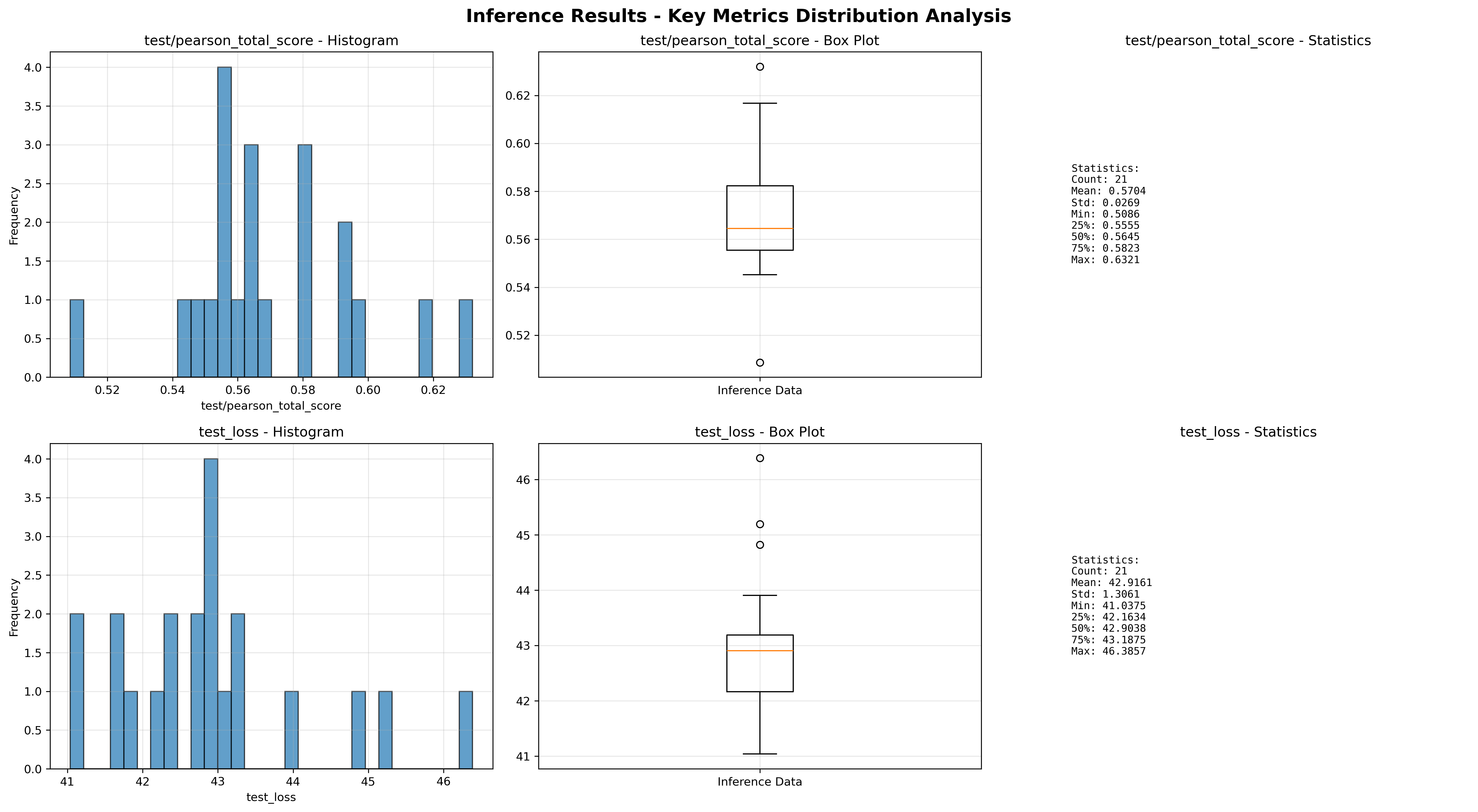
Once training was completed, the model variants were evaluated using validation data. Due to the training set misconfiguration, the models themselves do not provide scientifically informative predictions, and as a result are only compared to each other for consistency. Training loss and Pearson total scores are shown in Figure 7.
Experiment 2: Global Protein Model Training
A second round of training was conducted utilizing a larger model architecture more suited to the “global” scope of the training data and consistent with the published models. The resources, utilities, and strategies implemented in the initial experiment were heavily re-used for this second experiment.
Model configuration
This experiment used a larger variant of the METL model, designed to capture a globally useful representation of protein structure and energies. It is larger than the METL-Local model used in Experiment 1 but similar in architecture, with 6 layers, 8 attention heads, embedding dimension 512, and feedforward width 2048, with 19.2M total parameters.
The “global” dataset, described above, was used for training this model.
Results
Training process
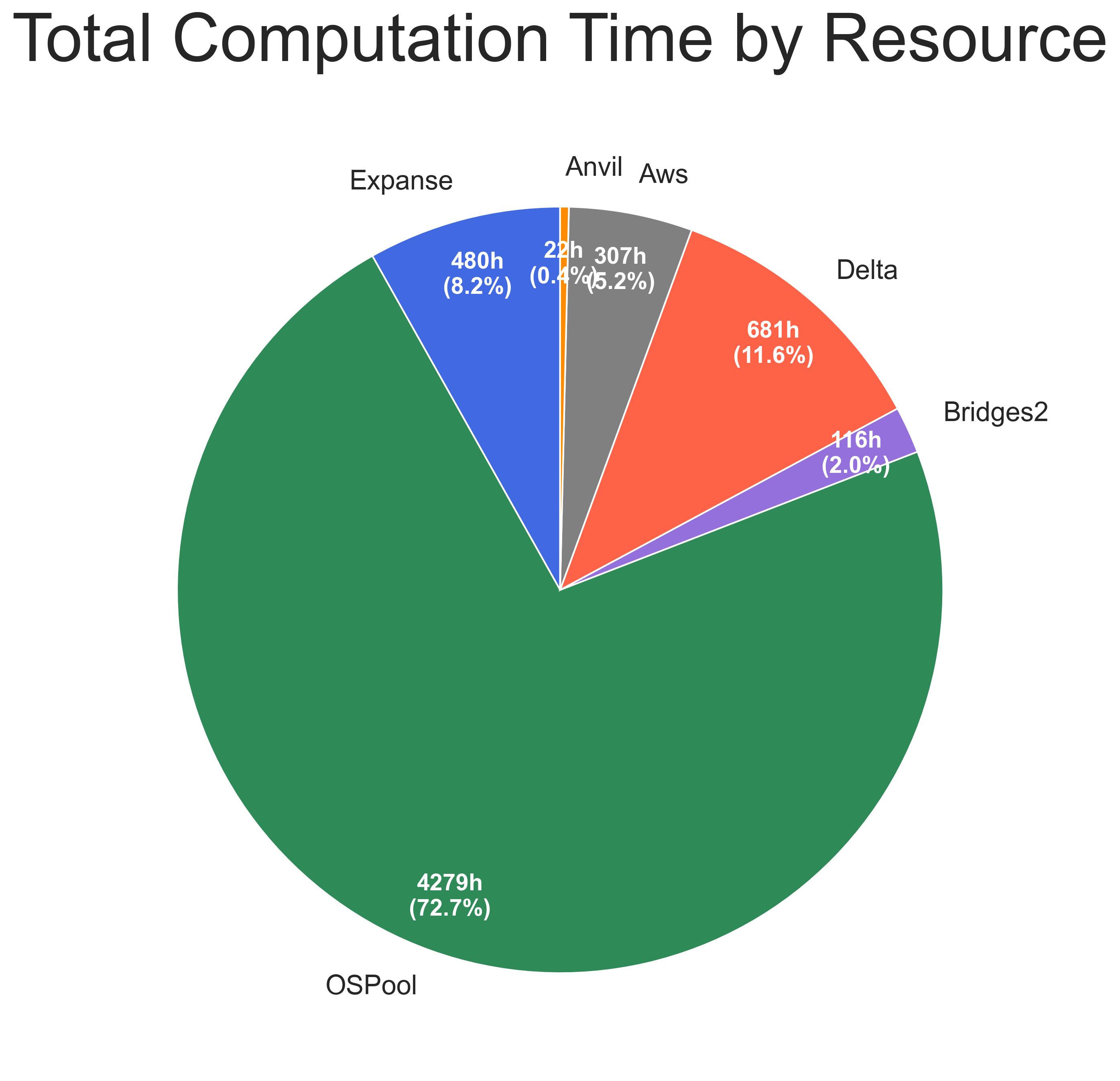
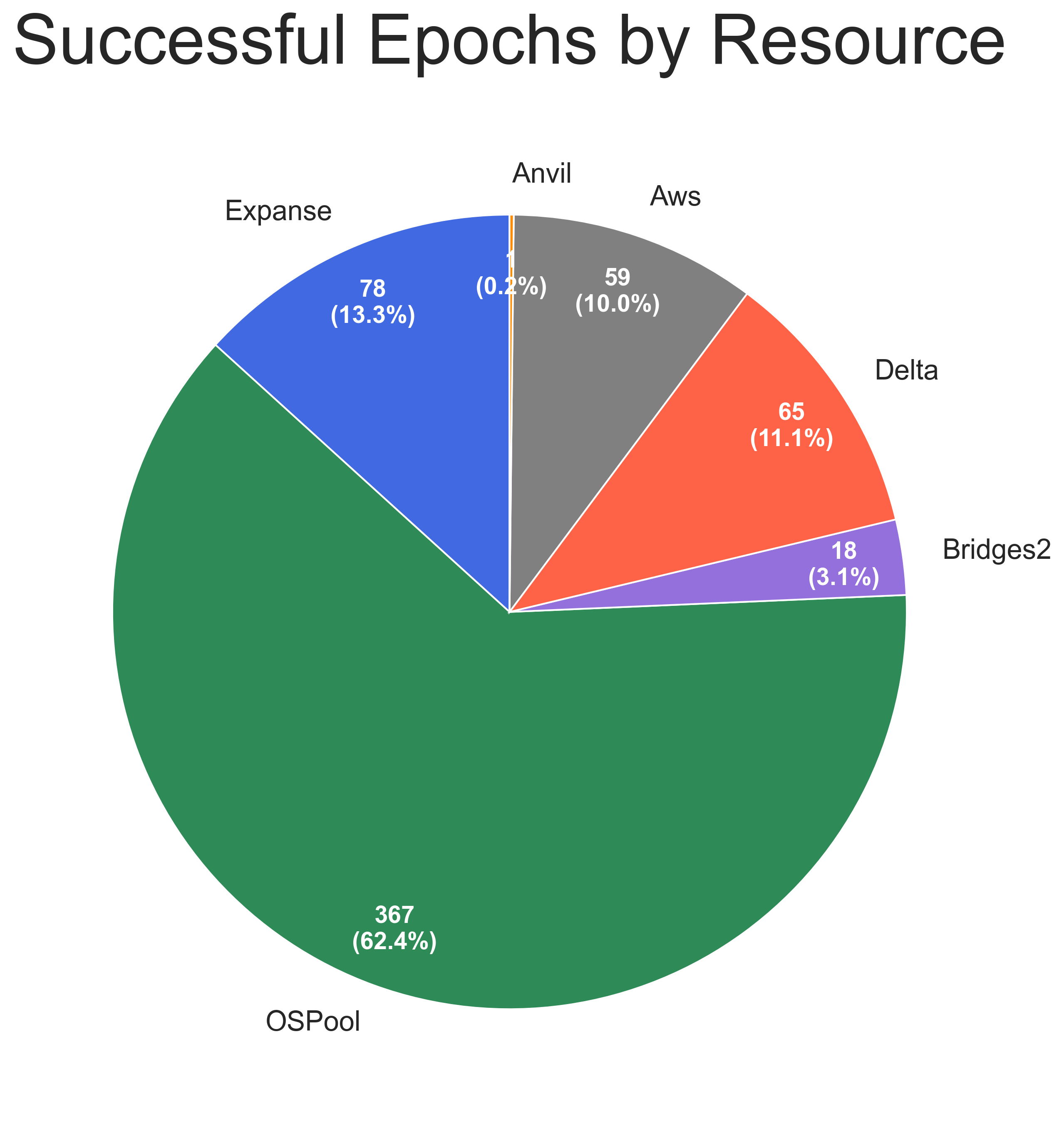
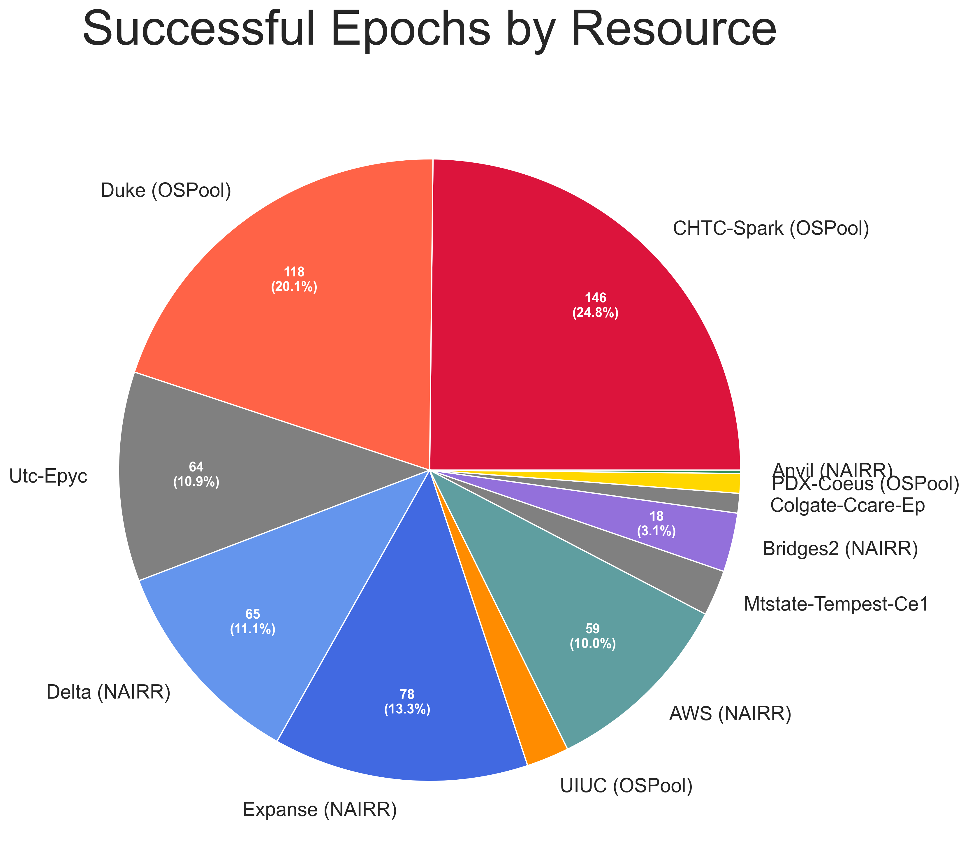
In total, 612 epochs were completed across five resources (OSPool, Delta, Expanse, Bridges-2, and AWS), consuming 20,045 GPU hours across eight GPU models.
| GPU Model | Epochs trained |
|---|---|
| NVIDIA A100 80GB PCIe | 64 |
| NVIDIA A100-SXM4-40GB | 61 |
| NVIDIA A100-SXM4-80GB | 135 |
| NVIDIA A40 | 37 |
| NVIDIA H100 80GB HBM3 | 47 |
| NVIDIA H200 | 121 |
| NVIDIA L40S | 55 |
| Tesla V100-SXM2-32GB | 92 |
GPU Utilization Breakdown — Experiment 2
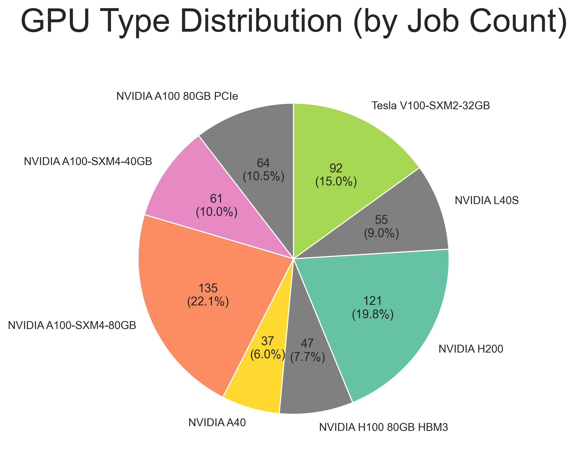
Evaluation
In addition to the heterogeneously trained models described above, reference models were also trained on the same dataset, constraining the training processes to a single GPU model type (or restricting the training to a single machine). These reference runs were smaller in scope, with 6 completed models and 264 total epochs trained.
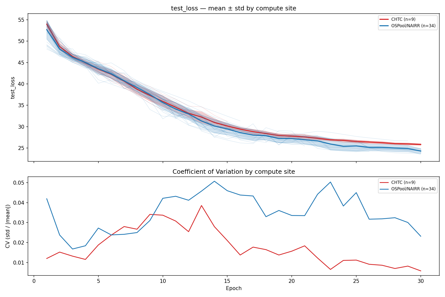
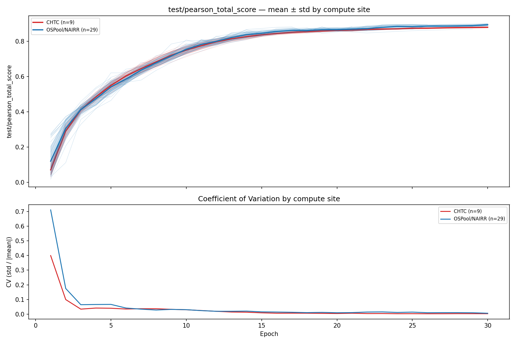
After each training epoch (in both the heterogenous and homogenous resource modes), the best-performing checkpoint seen so far (selected by validation loss) was evaluated on a held-out test set. Results were written to a per-epoch metrics file recording test loss and Pearson correlation coefficients between model-predicted and reference values for 55 structural and energetic properties. These include Rosetta all-atom energy terms, structural descriptors, and centroid-mode energy terms. An aggregate pearson_total_score summarizing overall predictive accuracy was also recorded each epoch.
To assess whether training outcomes differed systematically by compute environment, we compared evaluation metrics across runs grouped by site of execution: CHTC (homogeneous GPU types) and OSPool/NAIRR (heterogeneous GPU types). For each site group, per-epoch metric values were aggregated across all runs, and the mean and standard deviation were computed at each epoch. A coefficient of variation (CV) was also computed as the standard deviation divided by the mean, providing a relative measure of variability for each training approach. These results are shown in 12 and 13 for test loss and Pearson total score, respectively.
Conclusions
General considerations
For a model of the local size (2.5M parameters), the OSPool is an excellent source of GPUs available for training. The limited system and video memory needs are easily available within capacity donated to the OSPool, allowing for efficient training and optimization. It was not atypical for up to a dozen epochs to be training simultaneously, allowing for substantial overall throughput in the training process.
The larger architecture, requiring >60 GB of video memory, also saw success in the OSPool, but throughput was substantially lower than the local model due to the lower availability of contributed resources meeting the higher requirements.
The NAIRR sites also contributed significant computing resources, but they were not as heavily utilized as the OSPool due to the challenges in creating uniform and consistent pressure for jobs to consume existing annexes. The shape of the overall training process (where epochs moved across sites, often with long gaps between re-visiting a NAIRR resource), meant that an annex usually retired before being re-utilized by additional jobs. This created a substantial bottleneck, as re-establishing the annex required manual intervention (due to the need for two-factor authentication). This could be alleviated by requiring re-use of the same site for consecutive epochs at the cost of the desired GPU heterogeneity.
The per-epoch performance of the training process was difficult to characterize, and similar hardware across different sites resulted in significantly different training times. Attempts to address performance variation through CPU/GPU ratio adjustments and data locality improvements yielded minimal gains, suggesting that differences in training times like come from factors beyond job-level resource configuration, such as network characteristics or CPU/disk hardware variations. Troubleshooting attempts included manually logging into the NAIRR sites and submitting the work directly to the SLURM clusters there (to eliminate potential HTCondor/Annex impact), moving data from the job directory to dedicated solid state diskspace before training, and modifying batch sizes.
An innate challenge to adaptation of existing training workflows into a new environment is the unfamiliarity and “black box” nature of the software, which substantially complicates the ability to understand and investigate significant behavioral differences in heterogeneous environments.
Comparison between heterogeneous and homogeneous training approaches indicates that both approaches converge to similar model performance, in both test loss and Pearson total score. However, the coefficient of variation indicates that the heterogeneous approach results in considerably higher variability across each epoch.
DAG generation and pattern repetition
A pattern that is often repeated in machine learning training is the need to run multiple training jobs with slightly differing configurations. Ensembles of models, including experiments such as this project, and hyperparameter tuning are common uses cases that fall into this category of high numbers of “shish-kebab” shaped workflows. Between training runs, variables or parameters may be altered in order to optimize the model’s performance, test model architecture behavior, or to generate a group of similar models for comparison.
While creating the DAG generation script, we considered shortcomings and areas for improvement in the HTCondor software, especially in its Directed Acyclic Graph manager (DAGMan). While programmatically creating a DAG in this fashion is not a challenging scripting task, it is largely left to individual researchers to re-implement similar patterns in order to capture desired behavior.
DAGMan provides handles that are useful for this kind of work, such as being able to assign VARS at the NODE level, which allows for easily changing parameters between training runs. However, this must be done at the level of individual nodes, resulting in a verbose overall DAG definition that cannot easily be updated if needed. DAGMan also provides a way to define a subdag, which allows for repeated shapes within the overall workflow, but again lacks the flexibility in changing VARS within repetitions of the shape.
Being able to define subdag- or region-define variables would simplify the overall structure of the DAG file, enabling more concise and maintainable DAG definitions. Finally, hyperparameter sweeps, a very common operation in ML training, involves systematic explorations of a phase space. DAGMan lacks the ability to easily program “sweeps” of values, such as letting a VAR run from 0.01 to 0.1 in steps of 0.01. Should that feature be added, concise DAG definitions for complex ML training workflows could easily be created and utilized, instead of multiple ala carte solutions being created by research groups.
A concise description of a DAG with SUBDAG repetition and sweeps could look something like:
train.subdag
PARENT {run}-train_epoch0 CHILD {run}-train_epoch1
PARENT {run}-train_epoch0 CHILD {run}-eval_epoch1
PARENT {run}-train_epoch1 CHILD {run}-train_epoch2
PARENT {run}-train_epoch1 CHILD {run}-eval_epoch2
VARS {run}-train_epoch0 epoch=1 a={a} b={b}
VARS {run}-train_epoch1 epoch=2 a={a} b={b}
VARS {run}-train_epoch2 epoch=3 a={a} b={b}

workflow.dag
GEN SUBDAG train_flow train.subdag a, b from
  0.01 to 0.1 by 0.01
  0.5 to 5 by 0.5
PARENT init CHILD train_flow
This defined a “shish-kebab” training subdag, with parent-child relationships defined between epochs (with sidecar evaluation nodes). a and b represent parameters that change between training runs but are consistent within each run. A GEN command will generate the overall workflow, letting the values of a and b run over their respective ranges. Finally, an initializing node (init, included but not defined) defines any initialization that needs to happen for the workflow as a whole and serves as a PARENT node to the training runs.
Annex readiness for distributed machine learning training
While HTCondor Annex provides a unified interface to HPC systems that provide NAIRR allocations, the particular challenge of intentionally shifting training between sites is somewhat at odds with the intended Annex goal of “bursting” into a single HPC site to provide additional short-term computing resources. Instead, there was non-constant pressure of jobs targeting each site, resulting in constant annex retirement and the need for re-identification (often with two-factor authentication) at each site to re-establish the annex and continue training. This prevented full automation of the training process, as manual intervention was often required. Constant pressure (for example, from targeting only one NAIRR resource) could certainly solve this problem, with HTCondor providing the organization and management aspects of the training run.
There was also a clear shortcoming in the HTCondor Annex and its inability to handle changes in the “known” HPC sites. A fundamental assumption in early development of the Annex was that the AP contained a static list of HPC resources and certain settings at each (for example, valid partition names, GPU types, and OS versions). Whenever a site changed these things, the annex would break and require development efforts to update these settings. Opaque and obscure errors (or silent failures) further complicated these issues, as it was often difficult if not impossible to sort out what or where the failures were: the observed behavior was simply that jobs did not run at the expected site.
A new version of the Annex is currently under development, which addresses these issues, with:
-
Improved logging and error propagation, in order to make it clear what stage of the process was failing (HPC job failure, failure to start the EP, failure to connect the EP to the AP, unexpected EP configuration).
-
Removal of knowledge at the AP. It is now expected that the user be familiar enough with the HPC site to understand how to run a job there. The HTCondor Annex creation process becomes the movement of a tarball containing the EP software to the HPC site, where it is unpacked, further configured (e.g. with site specific credentials and requests), and submitted to the HPC scheduler.
Provenance tracking improvements
As part of an additional set of local protein model trainings intended to show a complete high throughput simulation → pre-training → finetuning chain of work, several changes have been made to the DAG generation software used in this work. Namely, an improved provenance tracking system has been implemented, which replaces the ad-hoc log-based scraping with a structured NDJSON event logging at all stages (DAG generation, submission, epoch start/completion, and job state transitions). Additionally, every checkpoint that is written retains a complete provenance side-car file, containing full provenance graph for that checkpoint. This information includes checksum, parent checkpoint checksum, host and GPU information, validation loss, and training time.
Future Work
-
Complete the local protein model training work into a full demonstration of a simulation → pre-training → finetuning chain, building on the provenance tracking improvements described above.
-
Adopt subdag- or region-scoped DAGMan VARS and a hyperparameter sweep syntax, as described in 6.2, to reduce the verbosity of ensemble and hyperparameter-sweep DAG definitions.
-
Continue rollout of the new Annex version (3.4) to resolve the logging, error-propagation, and static-site-configuration issues identified in this project.
Acknowledgements
This research is supported by the National Artificial Intelligence Research Resource (NAIRR) Pilot. The Anvil supercomputer is supported by the National Science Foundation (award NSF-OAC 2005632) at Purdue University. The Bridges-2 system is supported by NSF award number OAC-1928147 at the Pittsburgh Supercomputing Center (PSC). The Delta advanced computing and data resource is supported by the National Science Foundation (award NSF-OAC 2005572).
Appendix: Data Flow
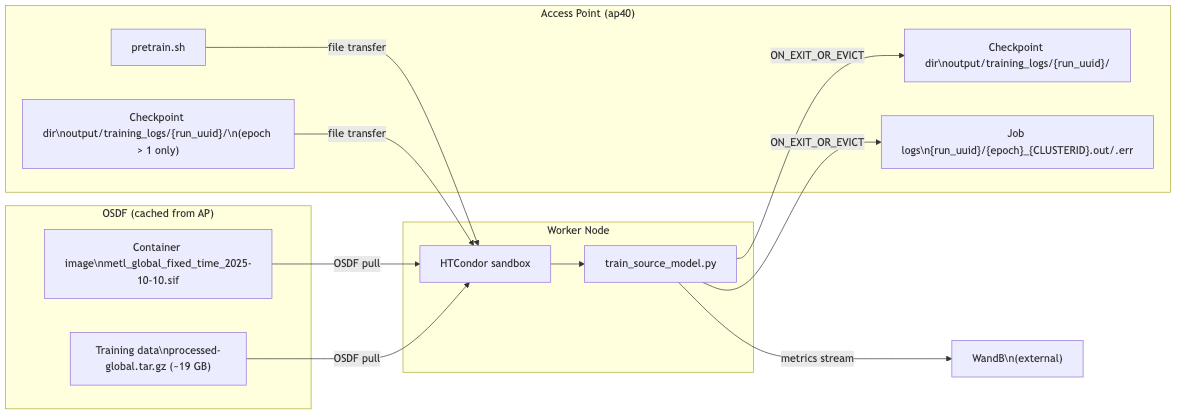
This appendix describes how data moves through the model training workflows. It covers what the data components are, where they are stored, and how they are moved into and out of computing nodes.
Overview
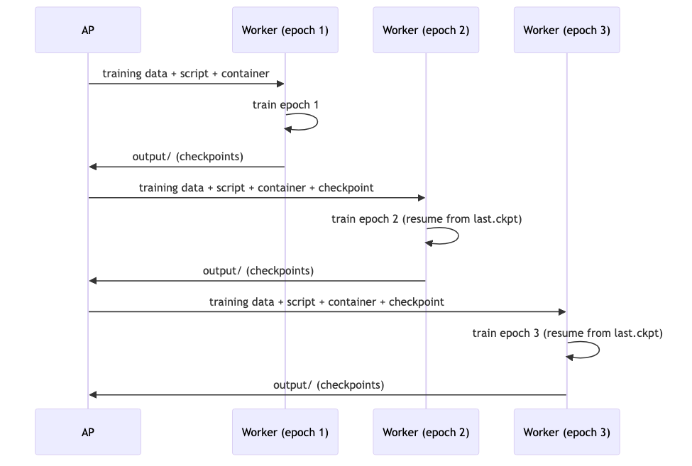
The DAG runs multiple independent training runs in parallel (e.g., run0, run1, run2). Each run trains a global METL source model for 30 epochs. Epochs within a run are strictly sequential: epoch N+1 cannot start until epoch N completes and its checkpoint is safely back on the AP. Across runs, there is no dependency — they proceed independently with different random seeds.
Each epoch is a single HTCondor job. Jobs can land on heterogeneous compute resources: glideins within the OSPool, or HTCondor annexes started within NAIRR sites (Expanse, Anvil, Delta, Bridges-2, and AWS). Barring minor resource request changes dependent on site particularities, the job description and data transfer are the same regardless of target.
Storage Locations
| Location | What lives there |
|---|---|
osdf:///ospool/ap40/data/ian.ross/ (Ceph via OSDF) |
Container image and training data, served via OSDF caching layer |
| ap40 working directory | pretrain.sh script, output/ checkpoint dirs |
| Worker node scratch | Ephemeral job sandbox during execution |
| Weights and Biases | Training metrics (streamed live during each job, if enabled) |
Storage locations for training artifacts
Inputs Per Job
Always transferred (every epoch)
| Artifact | Size | Source | Mechanism |
|---|---|---|---|
Container image (metl_global.sif) |
5.7 GB | Ceph via OSDF | OSDF pull |
Training data (processed-global.tar.gz) |
19 GB | Ceph via OSDF | OSDF pull |
Training script (pretrain.sh) |
1 kB | AP working dir | HTCondor transfer |
Artifacts transferred on every epoch
Conditionally transferred (epoch > 1)
| Artifact | Source | Mechanism |
|---|---|---|
Checkpoint directory (output/training_logs/{run_uuid}/) |
AP working dir | HTCondor transfer |
Artifacts transferred conditionally (epoch > 1)
The checkpoint directory contains .ckpt files (one per completed epoch, keyed by epoch/step/val loss) plus last.ckpt and a time_checkpoints/ subdirectory used for mid-epoch eviction recovery. The METL training software resumes training from the “best” checkpoint so far, falling back to last.ckpt when the best checkpoint was not successfully transferred to the AP. This occurred due to quota constraints on the AP: last.ckpt could be updated in place, but the epoch-specific file could not be written.
Outputs Per Job
| Artifact | Size | Destination on AP | Contents |
|---|---|---|---|
output/{run_uuid}/checkpoints/ |
230 MB | AP working directory | .ckpt files, last.ckpt |
| HTCondor stdout/stderr | ~20 MB | {run_uuid}/{epoch}_{CLUSTERID}.out/.err |
Job logs |
| HTCondor log | — | metl.log |
Lifecycle events |
| Metrics | ~20 MB | WandB (external) | Loss curves, learning rate |
Artifacts produced per epoch job
After all 30 epochs complete, the final checkpoints for a run are at output/training_logs/{run_uuid}/checkpoints/ on the AP. Completed runs are also synced via cronjob on the AP to Ceph storage (/ospool/ap40/data/ian.ross/global_checkpoints/) for redundancy.
What Happens on the Worker
-
HTCondor unpacks the job sandbox. The container image is already cached (or pulled via OSDF).
-
pretrain.shruns inside the container:-
Untars
processed-global.tar.gzintoglobal/, then deletes the tarball to reclaim disk space. -
Symlinks code in the container image (
/workspace/metl/data/) to the working directory. -
Runs
train_source_model.pywith hyperparameters stored within the container image at/workspace/metl/args/pretrain_global.txt, passing epoch number,run_uuid, and random seed.
-
-
Training streams metrics to WandB via API key set in the job environment.
-
On completion or eviction, HTCondor transfers the
output/directory back to the AP.
Other Notes
Each run’s checkpoints directory was periodically manually pruned to minimize movement of unnecessary epoch checkpoint files, as early weight files soon become obsolete in the training mechanism.
Data Flow Diagrams
Per-epoch job data flow
Epoch-to-epoch checkpoint chain (within one run)
References
-
Gelman, S., Johnson, B., Freschlin, C. R., et al. (2025). Biophysics-based protein language models for protein engineering. Nature Methods, 22(9), 1868–1879. https://doi.org/10.1038/s41592-025-02776-2 ↩
-
Gelman, S., D’Costa, S., Romero, P., & Gitter, A. (2025). METL Rosetta datasets [Data set]. Zenodo. https://doi.org/10.5281/zenodo.14916528 ↩
-
Kurtzer, G. M., cclerget, Bauer, M., Kaneshiro, I., Trudgian, D., & Godlove, D. (2021). hpcng/singularity: Singularity 3.7.3 (Version v3.7.3) [Computer software]. Zenodo. https://doi.org/10.5281/zenodo.4667718 ↩
-
Leaver-Fay, A., Tyka, M., Lewis, S. M., et al. (2011). Rosetta3. Methods in Enzymology, 545–574. https://doi.org/10.1016/b978-0-12-381270-4.00019-6 ↩